2018-19 Season in Review: Montreal Canadiens & Ottawa Senators

By Constantine Maragos

This year, the Eastern Conference was stronger than ever, with powerhouses such as the Tampa Bay Lightning leading the league throughout the regular season, along with playoff mainstays in the Washington Capitals and Pittsburgh Penguins. The Montreal Canadiens and Ottawa Senators both fell to the same fates at the end of this year, missing the post-season in back-to-back years. However, both franchises followed very different storylines throughout the year, yet both have promising futures going forward.

Montreal Canadiens

The Montreal Canadiens catapulted themselves back into the playoff conversation this season and finished off a respectable 2018-19 campaign with 44 wins and 96 points, placing them 4th in the Atlantic and 14th in the league. Despite falling two points short of the playoffs, the Montreal Canadiens showed signs of true growth, while also mending some of their biggest issues over the past few seasons. The Canadiens’ improvement this season can be attributed to a combination of the return to form of veterans such as Carey Price & Shea Weber, an injection of youth into the lineup, and a number of shrewd acquisitions by GM Marc Bergevin.

The key acquisition that Montreal made this summer was swapping former 2012 3rd overall pick Alex Galchenyuk for Arizona’s Max Domi. After struggling to find an effective top-six centre, Max Domi seemed to fit into that role well this season. Despite Domi’s rough start to his Canadiens’ tenure, receiving a preseason suspension for his sucker-punch on Florida’s Aaron Ekblad, Domi has settled in nicely with the Habs. Domi’s 28 goals and 72 points this season place him first in team scoring. In addition, his 0.88 all-situation xGoals/60 is good for fourth among Canadiens forwards. Also, his hard-hitting, pesty play style has led to an average of 3.14PIM/60, but while also drawing 3.25/60 penalties as well, leading Canadien’s skaters in both categories. Domi’s enigmatic playstyle has drawn mixed reviews, however, if he can turn this season’s 28 goal, 72-point performance into the standard of performance going forward, Habs fans will not be complaining too much in the future.

The return of captain Shea Weber gave the Canadiens an injection of veteran leadership and much-needed skill on the back end after the defenseman was sorely missed last year. Weber made his return known across the league after scoring 2 goals and 3 points in his first two games and has stabilized the Habs’ back end since. His 14 goals and 33 points this season are good for second in goals & points among Habs defensemen behind only Jeff Petry. Carey Price experienced a return to form this year, going 35-24-6 in 64 starts while posting a 2.49 GAA along with a 0.918 SV%, good for 12th in each category (among goalies with >25 GP). Price also finished 3rd in Quality starts with 37, as well as placing 8th in Goals Saved Above Average with 14.94. Additionally, Tomas Tatar was a pleasant surprise for the Canadiens. Having been shipped to Montreal in the summer in a package for former captain Max Pacioretty, Tatar carried with him the baggage of an underperforming contract. Tatar took his fresh start opportunity and ran with it, scoring 25 goals and 58 points on the season. Further, he finished the season with 0.84 xGoals/60 at 5v5, good for 5th amongst forwards. As a staple in the top six, Tomas Tatar has found himself a home in Montreal.

The Achilles heel in the Canadiens lineup was the struggles of the fourth line. The rotating carousel of Michael Chaput, Kenny Agostino, Nicolas Deslauriers, Charles Hudon, and Matthew Peca struggled immensely throughout the year. To note, the group’s possession metrics had been abysmal. In 5v5 relative Corsi, Deslauriers, Hudon, Chaput, and Peca round out the bottom for forwards, all sitting below -3.8%. To put things into perspective, the Ottawa Senators had only two forwards (with >20 games played) with a sub -4% relative Corsi. Additionally, apart from Kenny Agostino (51.6%), each player finished sub-50% in On-Ice xGoals/60. Only two other players on the roster finished in this category. With these struggles in mind, Marc Bergevin made two moves in an attempt to fix the problem. The Canadiens acquired Nate Thompson & a 2019 5th round pick from LA for a 2019 4th round pick, as well as Dale Weise & Christian Folin from Philadelphia for AHL forward Byron Froese and depth defenseman David Schlemko (both trades occurring in February). Along with these acquisitions, the Canadiens subsequently waived Michael Chaput and Kenny Agostino, who was claimed by the New Jersey Devils. However, Nate Thompson did not make much of an impact initially with the team, as he posted comparable advanced statistics as the players listed above, but did play well enough down the stretch to earn himself a one-year/$1 million extension. In addition, Dale Weise jumped between AHL Laval and the Canadiens’ press box since his acquisition. However, at the Trade Deadline, Bergevin flipped the recently waived Chaput to the Arizona Coyotes in exchange for winger Jordan Weal. Jordan Weal fit nicely into the Habs’ bottom six after shuffling around the league this year. Since joining the team, Weal has scored 4 goals and 10 points in a fourth line role. Additionally, he logged 1.4 even strength points/60, a higher total than each of the above-listed names. Weal also allowed the least amount of shot attempts Against/60 on the roster at 50.62. Weal’s performance down the stretch earned himself a two-year/$2.8 million extension. Despite the small sample size, the Habs looked to have found a few upgrades in the bottom six going into next season.

Looking forward, the Canadiens’ future looks bright. Centre Ryan Poehling looks like he is going to be a staple in the centre of the Habs lineup for years to come. Poehling made quite the first impression in his first career game, scoring a hattrick and the shootout winner against the Toronto Maple Leafs no less. Jesperi Kotkaniemi experienced ups and downs this year as a first-year player but also looks to be a future mainstay in the Habs' lineup. If Marc Bergevin is able to find a solution to their fourth line issues, while their young core continues to produce next season, the Canadiens look set to enter the playoff conversation next year.

Ottawa Senators

For the past two years, the Ottawa Senators organization has been mired in controversy, questionable moves, and subpar play. After trading away estranged captain Erik Karlsson to the San Jose Sharks, the Senators we left without an identity going into the 2018-19 season. The Senators finished off a dismal campaign with 29 wins and 64 points, leaving them at the basement of the NHL standings. Along with their last-place finish, the Senators will be without their first-round selection, now the fourth overall pick in this year's draft. Despite finishing as the worst team in the NHL, the Senators are still able to take some positives from this year. 

If the Senators were to take anything away from this season, it would have to be the emergence of Thomas Chabot. Chabot’s breakout 2018-19 campaign finished with 14 goals and 55 points, placing him 10th in NHL scoring among defensemen, while also missing 12 games due to two separate injuries. In addition, Chabot was selected as the Senators’ All-Star participant in San Jose. This year Chabot displayed the untapped potential that he possesses and looks poised to lead the Senators into their franchise’s next chapter. Chabot was an all-situations player for the Senators, logging around 20:45 even strength minutes per game, ranking 4th in the NHL behind only Seth Jones, Ryan Suter, and Drew Doughty. As a 22-year old defenseman, being mentioned among such prominent names is a great sign for things to come.

As the Senators began to fall out of playoff contention, the chatter of moving pending free agents Matt Duchene, Ryan Dzingel, and Mark Stone ramped up tremendously. Against the preconceived notions of many, GM Pierre Dorion was able to get solid value for the three veteran forwards. In a flurry of trades with the Columbus Blue Jackets, the Senators traded (in total) Matt Duchene, Ryan Dzingel, and Julius Bergman for Anthony Duclair, Vitaly Abramov, Jonathan Davidsson, a 2019 1st round pick, a 2020 conditional 1st (contingent on Duchene re-signing), a 2020 2nd round pick, and a 2021 2nd round pick. Given the position Dorion was in, he seemed to have yielded a solid return. With Columbus’ pending free agent situation taken into consideration, the draft picks Dorion received may significantly rise in value. In addition, Anthony Duclair has been a pleasant surprise for the Senators, having been considered a "throw-in" in the Dzingel trade, Duclair has scored 8 goals and 14 points in 21 games with the Sens, more than both Dzingel and Duchene in those categories. While Duclair’s xGoals/60 stayed relatively constant at ~0.8, since leaving Columbus, Duclair’s on Ice xGoals/60 rose from 2.4 to 9.99, which is again a big jump from the pair sent the other way. After jumping around the league for the past few years, Duclair may have been able to find some consistency and confidence on the Sens roster.  

The Senators also traded star winger Mark Stone in a blockbuster to the Vegas Golden Knights for blue-chip prospect Erik Brannstrom, a 2020 2nd round pick, and forward Oscar Lindberg. The 15th overall selection in the 2017 Entry Draft is developing into a superb offensive defenseman. As an AHL rookie, Brannstrom scored 7 goals and 32 points in 50 games. Brannstrom was also named an all-star at the 2019 World Junior Championship, scoring 4 goals in 5 games at the tournament. Although Mark Stone is a tremendous talent, and one of the best defensive forwards in hockey, Ottawa Senators fans should be excited for what’s to come with the likes of Erik Brannstrom and Thomas Chabot leading the backline.

Looking forward, the Senators have a lot of talent up front in chippy forward Brady Tkachuk, and young centre Colin White, among others. Additionally, with Thomas Chabot continuing to grow into a superstar, and Erik Brannstrom converting his solid offensive game to the NHL level, the Senators are well prepared as they move forward in their rebuild. Although it remains to be seen whether their decision to pick forward Brady Tkachuk over whoever is available with Colorado's fourth-overall pick this year, the Senators have been able to recuperate draft picks to help mend the difference. The Senators will still have a full seven draft picks this season, including four in the first three rounds. Furthermore, the Sens have 12 draft picks in 2020, including 7 in the first three rounds, and 8 draft picks in 2021. Despite the external uncertainties surrounding the Senators for a multitude of reasons, the organization needs to move on. For the Senators organization to move on from the circus that has been the past two years of their franchise, the front office needs to concentrate on the future and draft smart. In doing so, the Senators may be able to regain the trust of the fanbase in the future.

Special thanks to Owen Kewell for this article.

Keep up to date with the Queen's Sports Analytics Organization. Like us on Facebook. Follow us on Twitter. For any questions or if you want to get in contact with us, email qsao@clubs.queensuca, or send us a message on Facebook.

Major League Baseball capacity rates: Analyzing fan attendance using panel data

By Cody Smith and Patrick Mills

A note from the article’s editor (Anthony Turgelis): This article will read somewhat differently from the rest of our content, as this was a detailed final project for a 4th year Applied Econometrics course at Queen’s. I hope you enjoy the format, as it is more typical for analytics research projects.

Introduction

            Major League Baseball has been recognized as a staple of American culture since its inception in 1869. Over generations, the League has transformed from humble beginnings into an organization with 30 franchises over North America each playing 182 games per season. This period has seen franchises experience different levels of success when attempting to attract fans to games, and this variation has drawn the attention of many Economists looking for an answer as to why. Ahn and Lee (2014) found that from 1904-1957, fans were captivated by teams with the most winning record. This period was followed by a change in preference which Ahn and Lee identified as a desire for competitive games (1958-2012). Now, in the modern era, sports fans have a variety of professional sports to watch, as well as the ability to follow and support teams from a distance thanks to increased media coverage and reduced costs of transportation. Similar to how companies in retail rely on branding to differentiate themselves and attract customers, it is likely that branding will become increasingly important for MLB franchises as they compete with a growing number of substitute franchises across sports to attract people to fill seats at games.  This paper will examine the effect of Brand Equity Value (BEV) on capacity rates across MLB franchises. Our computation of BEV will be explained in our description of data. If the relation between BEV and capacity rates is found to be statistically significant, it could have major implications as it would provide compelling evidence of a new shift in fan preferences. Franchises would have to choose how to market themselves to stimulate interest among local and distant baseball fan bases alike. Evidence for a shift in fan preferences would also provide considerations for the MLB when creating policy to promote and protect the league’s growth and popularity.

            The remainder of this paper will be structured as follows: The second section will provide a commentary on existing literature discussing factors of MLB attendance. The third section will describe from where the data used in this paper as well as provide further explanation of BEV. The fourth section will explain the empirical model used in our regression analysis, as well as why it was chosen. The fifth section will present our regression tables as well as a commentary on the results. Finally, the sixth section will conclude with a summary of this papers findings as well as the importance and implications of these results.

Literature Review

Economists have published a collection of articles speculating over the key determinants of attendance for Major League Baseball franchises. Nesbit and King (2012) released a report finding that fans who play fantasy baseball are more likely to attend games, while Mittelhammer, Fort, et al., (2007), found increasing proximity between teams had an adverse effect on attendance in accordance with Hotelling’s model that consumers buy goods from the closest supplier. Ahn and Lee (2014) concluded that in earlier years of baseball (1904-1957) fans had been drawn to teams with winning records – the better the record, the higher the turnout – before a new era of baseball (1958-2012), saw fans who were drawn to games based on uncertainty of outcome, size and quality of the stadium as well as the playing styles of the teams. Throughout the literature however, one overarching determinant became reoccurring: the maintenance of a competitive balance in the league. Berri and Schmidt (2001) investigated this matter and concluded that as the league became more competitive, attendance could be expected to increase. Lemke, Leonard, et al. (2010), who attempted to establish a relation between promotions and giveaways in small and large markets on attendance, found competitive balance to be a significant factor of attendance. Ahn and Lee (2014), reached the same conclusion as well. Economists approaching the subject seem to agree that competitive balance is essential to the interest of fans as well as the financial health of the league. Lee (2016), showed that fans consider characteristics of home and away teams when making attendance decisions. In the same report, Lee also hypothesized that modern era baseball fans had less incentives to cheer for the home team, citing development of media and greater access to information, mobility in residence and reduced transportation costs as factors that would allow fans to pick and choose a team they wanted to support, rather than teams in close proximity. While this is still consistent with competitive balance, if true, previous methods of incentivizing local fans to attend games would prove to be less efficient.

Description of Data

            The primary data that was utilized in our regression model was obtained from ESPN, Sports Reference, Statistics Canada, Statista and the United States Census Bureau. Supplementary information used from Boston Globe Media Partners examined MLB ticket prices, and this paper took data presented by Forbes Media to establish franchise valuations. Data from ESPN and Sports Reference provided information on stadium capacity rates, strength of schedule, win rate over .500, estimated payroll, homeruns per game, and pace of games. The United States Census Bureau and Statistics Canada data pools were used to establish the demographic parameters of population and median household income. Data from Statista was referenced to establish ticket prices. We also took into consideration the addition of professional sports teams to cities with MLB franchises by including a dummy variable. If these arriving franchises were a part of a big four league (NHL, NFL, NBA, MLB), the existing MLB franchise was given a value of 1, while MLB teams in cities that did not gain a professional team were given a value of 0. Those that lost a franchise were given a value of -1. We also assigned a dummy variable to account for MLB franchises that moved into a new stadium over the period of examination. Teams that moved were assigned a value of 1 while teams that did not were assigned a value of 0. It is important to note that this is a potential source of error in our paper as teams who moved from a larger stadium to a smaller stadium will have experienced an increase in stadium capacity rate without a real increase in game attendance. Data from these sources was used to collect relevant information from all 30 MLB teams in the years 2008 and 2018, with a total of 60 observations.

Our primary measure deals with the evaluation of brand equity and is represented by the variable BEV. To accurately quantitate this qualitative statistic, we standardized four separate variables and used the average of the values to compute each franchises BEV statistic. As we only took data from separate two years, it was only possible to determine the effect of BEV in 2018. These four variables used for our BEV statistic are as follows:

1.      Market share – Presence in the market (2018 season)

a.       % of market share per team

b.      Individual team valuation/Sum of MLB team total valuation

2.      Transaction value – Price offered for service (2018 season)

a.       Average ticket prices/team

3.      Success generation – Team performance change (2008-2018)

a.       (Win % 2018 season/Win % 2008 season)-1

4.      Growth rate – Team valuation change (2008-2018)

a.       (Team valuation 2018 season/Team valuation 2008 season)-1

Table 1. Definition of Variables

Figure 2. Summary Statistics

Empirical Model

            To estimate the determinants of capacity rate, we have chosen to use a panel data regression. To decide between a fixed effects and random effects model, a Hausman test was conducted. After our results yielded Prob>Chi2= > 0.05, we chose to use a random effects GLS regression. This method will allow us to compare common factors of short-run demand to determine capacity rates in our given seasons, 2008 and 2018.

Equation (1) presents our basic empirical model of MLB game attendance:

Table 1 included in our description of data provides an explanation for each variable included in our empirical model. Using a random effects model is this instance is useful as the variation across franchises in our model is assumed to be random and uncorrelated with the predictor or independent variables included. Random effects assume that the error term is not correlated with the predictors, and under this assumption a random effects model will produce unbiased estimates of the the coefficients, use all the data available, and produce the smallest standard of error. After running our random effects GLS regression, we ran a simple OLS regression to determine how much of the variation in capacity rates could be explained by our Brand Equity Value variable, BEV, which will serve as our primary parameter of interest.

Results and Discussion

            After running our random effects GLS regression, we found three variables to be statistically significant. They were: estimated payroll for the season, home runs per game and franchise value. Our R-squared was 0.6407, and shows a strong correlation between the effect of the variables on the capacity percentage for MLB teams.

After running this regression, we tested our BEV statistic against the 2018 results to determine how much of the effect could be could attributed Brand equity value.

We found BEV to be statistically significant, with an R-squared value of 0.5196, meaning that 52% of the change in capacity percentage across MLB franchises can be accounted for by our constructed BEV variable. To the best of our knowledge, this paper is the first Economic evaluation of the effects of Brand Equity on capacity percentage, which is a direct measure of fan demand for a franchise. Our findings from our random effects GLS regression were consistent with existing literature, as estimated payroll, homeruns per game and franchise value have consistently been significant indications of attendance.

Conclusion

            The purpose of this paper was to establish an understanding of the impact of different variables on the capacity rate of MLB franchises. We took a collection of data from the 2008 and 2018 MLB season, as well as corresponding data of demographics and ran a random effects GLS regression, followed by a linear regression to determine how much of the change in capacity rates could be explained by our variable of interest, BEV. We found three variables in our random effects model to be statistically significant: estimated payroll, homeruns per game, and franchise value. Our findings in this regression are consistent with the literature. The results of our linear regression proved our hypothesis that Brand Equity Value plays a statistically significant role in determining capacity rates for franchises across the MLB. These findings are important as they indicate that fan preferences may be changing again, which is an observation that has been made in the literature over different periods. A change in fan preferences will have implications relating to economic and policy decisions as franchises attempt to stimulate fan interest by providing different amenities and incentives to differentiate themselves from the competition. The success of these efforts has implications for the municipalities and regions that generate tax revenue from the operations of these franchises, and could impact future decisions regarding expansion and relocation of MLB franchises.

NHL Western Canada 2018-19 Season Recap

By Constantine Maragos

With the conclusion of the 2018-19 NHL season, the Edmonton Oilers and Vancouver Canucks are facing the year-end media earlier than they’d like. Both teams have young superstars taking the league by storm, however glaring issues in each team holds them back from taking the next step. In this article, we’ll look into each of Edmonton and Vancouver’s seasons and look to see where they excelled, and where they need to improve.

Edmonton Oilers (35-38-9), 7th in Pacific Division

The Edmonton Oilers have caught themselves in another lacklustre season after their second round, seven-game series against the Anaheim Ducks two years ago. This year has been especially disappointing for the team. The Oilers finished with 35 wins and 79 points, good for 7th in a relatively weak Pacific Division, and 25th overall in the NHL. There is a multitude of factors one could blame this season’s finish for, including asset mismanagement and an underperforming roster.

Former Oilers General Manager Peter Chiarelli made a number of questionable moves in his tenure with the team that we do not need to harp on more than they already have. However, in the scope of this Chiarelli made certain moves which left the Oilers in the same position, or worse. To start, roughly one month into the season, the Oilers swapped Ryan Strome for New York Rangers forward Ryan Spooner. After only scoring 2 points in his first 18 games, it made sense at the time to try and shake things up with the swap. However, in doing so the Oilers acquired a player who’s struggles went beyond the offensive end. Spooner’s subpar defensive ability has been well documented and has led to his movement around the league. On the other hand, with a decreased defensive usage with the Rangers, Strome has been able to score at a significantly higher level. Spooner did not manage to score any more than he did in New York. Shortly after Chiarelli’s release, the new Oilers regime sent Spooner to the Canucks for Sam Gagner, who has been itching for NHL time since being stuck with the AHL Marlies all season. Gagner has been a step up from what Spooner and Strome were for the Oilers, recording 10 points in 25 games for the team.

The other two moves Chiarelli made this season involved shipping off forward Drake Caggiula, Jason Garrison, & a 2019 3rd round pick in a pair of trades to acquire defensemen Brandon Manning from the Blackhawks and Alex Petrovic (0-1-1, -7, 9GP) from the Panthers (both trades happened on December 30th). Again, these trades seem to have been poor asset management. Brandon Manning played a total of 12 pointless games for the Oilers before he was assigned to AHL Bakersfield. Alex Petrovic did not fare well either, playing only nine games, although he did miss time due to injury. As an impending UFA Petrovic did not make much of a case to be re-signed. Through his nine games with the team, Petrovic recorded only 1 assist, and registered a -7 plus/minus. Petrovic also achieved a -10.1% relative xGoals, as well as sitting at an On-Ice Shot Attempts Against/60 of 62.07. Petrovic served as a healthy scratch from February 16th until the end of the season. In turn, Drake Caggiula (5-7-12, +3, 26GP) stepped up his play with the Blackhawks. Although Caggiula has not been anything near a revelation, the primary scrutiny surrounding these moves is the lack of asset management and desperation shown by management. Of course, such moves are not the primary factor the Oilers’ demise but can be looked at as a sample size of the countless missteps that have occurred over the years. With many needs to address this season, the incoming management regime is left with a slim talent pool, and many needs to address this offseason.

Apart from the number of media storylines that shadow the organization, Leon Draisaitl enjoyed a career year. There was no shortage of critics regarding the huge contract he signed in 2017. Draisaitl’s 8-year/$66 million contract accounted for 11.33% of the Oilers cap hit at the time (and caused plenty of headaches among Leafs fans earlier this year), however, he has certainly begun to live up to that number, if not already. Draisaitl finished the year with 51 goals and 105 points, placing him 1 goal behind Alex Ovechkin for the Rocket Richard trophy and 4th overall in scoring. Draisaitl was also tasked with a heavy workload throughout the season, averaging 22:35 in ice time, second only behind teammate Connor McDavid among forwards. This statistic alone should measure the importance of these two players to the Oilers roster.

The most intriguing storyline this season was the persistent speculation surrounding 20-year old forward Jesse Puljujarvi. Puljujarvi never solidified himself into the Oilers lineup. To summarize Puljujarvi’s struggles this season, agent Markus Lehto has stated that it “may be beneficial [for Puljujarvi] to go somewhere else.” With that being said, assessing Puljujarvi’s current value is tough, as he is only 20, and a fresh start is what he may need. With only 4 goals and 9 points through 46 games, Puljujarvi’ season ended on February 15th due to a hip injury, which he underwent surgery for on March 4th. However, through such low production and inconsistent play Puljujarvi has not shown that he is capable of becoming a full-time NHL player. But as he is so young, the Oilers need to assess whether or not it is worth keeping someone who has shown flairs of skill or cut their losses and move forward with other assets. It is also worth mentioning that Edmonton has set a high price for Puljujarvi at a 1st, a prospect, and another asset (per Darren Dreger). It remains to be seen how the situation will play out, but the most sensible trade scenario, given Puljujarvi’s play and trending value, would be to try and swap him for another young player in a similar situation.

Looking forward, the Oilers have many needs to address, whether it be finding depth on the wing or stability on defense. The only consistency that lies within the organization is their two stars in Connor McDavid and Leon Draisaitl who seem to score no matter the circumstance. If the Oilers want to compete soon, they will need a number of smart acquisitions astute player development to improve their fortunes next year.

Photo credited to Anne-Marie Sorvin — USA TODAY

Vancouver Canucks (35-36-11), 5th in Pacific Division

Despite playing at around .500 for the entire season, the Canucks found themselves playing some meaningful games up until near the end of the season. The Canucks finished with 35 wins and 81 points, placing them 5th in the Pacific Division and 23rd in the NHL. However, without the outstanding second-half of Jacob Markstrom, the emergence of young superstar Elias Pettersson, and the reliable defensive play of centre Bo Horvat, the Canucks would be in a much lower place in the standings.

Through 60 starts this season, Jacob Markstrom posted a 28-23-9 record. The Canucks starter also contributed 34 Quality starts on the season, as well as an 11.1-point share, tied for 7th in the league. However, his performance in the second half of the season was a catalyst in keeping the Canucks near the playoff conversation this season. Since December 7th, Markstrom posted 19 wins at a 0.921 SV%, paired with his one shutout for the season. Night in and night out, Markstrom provided the Canucks with an opportunity to win. One of his most notable performances of the season was his 44-save outing in February against the fully-loaded Calgary Flames. The Flames outshot the Canucks 34-13 in the second and third period, but Markstrom held his ground throughout and led the team to a shootout victory. The progress Markstrom has made this year gives the Canucks needed stability in net throughout the rest of their rebuild, as rookie netminder Thatcher Demko still needs time to develop into a full-time pro, and prospect Mike DiPietro is still multiple years away from the Canucks crease. Going into next season, if Markstrom is able to build off his play this season, the Canucks could be playing meaningful games in spring quicker than we’d expect.

Another popular storyline is Elias Pettersson’s record-breaking season. The Swedish rookie hit the ground running at the beginning of the 2018-19 campaign, scoring in his debut, and subsequently scoring 10 points in 10 games through the month of October. Pettersson finished the season with 31 goals and 66 points, leading not only the Canucks but the entire rookie class in scoring by a considerable margin. Pettersson set a multitude of records through his impressive feats this season, most notably setting the record for most points by a Canucks rookie. In addition, the Pettersson effect was alive and well throughout the season. Petterson ranked third in relative Corsi at 4.3%, only behind linemates Brock Boeser and Josh Leivo no less. Despite complaints regarding his size (or lack thereof) Pettersson’s ability this year to protect and handle the puck in such a skilled manner has reinvigorated the Canucks offense. The insertion of Pettersson into the Canucks lineup has allowed for a seamless transition into a new identity for such a young core and gives great hope for the future. The next step in Pettersson’s career is his forthcoming Calder trophy win. However, a slow finish to the season and explosive entrance into the league by 25-year old rookie Jordan Binnington has created a bit of a conversation. Nonetheless, expect Pettersson to be named rookie of the year, and improvement next year on his already spectacular game.

As injuries seem to plague the Canucks year after year, head coach Travis Green leaned on centre Bo Horvat tremendously throughout various stretches of the season. Injuries to bottom-six centres Brandon Sutter and Jay Beagle at the beginning of the year led to a tremendous defensive load for Horvat to manage. Tasked with shutting down the top opposition night in and night out, while also looked at to still produce, Bo Horvat showed how important he is to the Canucks roster. Horvat lined up for 2018 faceoffs on the year which is more than any other player in the NHL. Additionally, 38.6% (779) of those draws came in the defensive zone. Horvat finished the year with a 53.7% success rate on draws. Along with the heavy defensive burden, Horvat had a career year offensively, recording career highs in goals, assists, and points (27-34-61, 82GP). As Horvat continues to develop as a 200-foot player, he has still yet to reach his full potential.

The biggest weakness that the Canucks have is their struggle on defense. Throughout the season, it was apparent that veteran Alex Edler was the backbone of their defense core and was relied on more than ever to perform. Edler logged an average TOI of 24:34, ranking him 10th in the NHL. Edler also missed extensive time due to injury, playing only 56 games on the year. The damage was tough to mitigate for the Canucks fdefense, as veteran Chris Tanev also missed a comparable amount of games this year (27). While this is not an unknown phenomenon, especially for Tanev, the absence of the veteran duo was missed more than ever. Despite the magnitude of games lost to injury, Edler was still able to produce impressive numbers, posting 10 goals and 34 points on the year. This was Edler’s 3rd time scoring 10 goals or more in a season, and the first time since 2011-12. As an impending free agent, and well-documented for his admiration of the city he’s called home his entire career, expect Edler to be back next season. As for the rest of the Canucks defense, there is still work to be done. Although defensemen Ben Hutton and Troy Stecher made good progress this year, there were countless occasions where they were anchored by defense partners such as Erik Gudbranson and Derrick Pouliot.  Before being traded, defenseman Erik Gudbranson was one of the worst possession defenders in the NHL. At the time of his trade, Gudbranson led the Canucks in shot attempts against per 60 with 66.64, while also at the bottom of the league in plus-minus at a -27. In addition, defenseman Derrick Pouliot looked lost at times when out on the ice. The lack of physicality from both defensemen led to long, drawn-out shifts in the defensive zone and countless turnovers on the breakout. Luckily, with the arrival of Quinn Hughes and potentially new personnel in the offseason, ice time on the back end will not be taken for granted, and play will improve.

Looking forward, the Canucks have a strong young core already in the NHL and will add another top prospect with the #10 pick at the NHL Draft in Vancouver. Also look for  Bo Horvat to take another step, where presumably he will be named team captain, a role that’s been he’s been groomed for ever since he came into the league. In addition, the developing chemistry between Brock Boeser and Elias Pettersson will only become stronger, and they have the potential to become one of the top duos in the NHL. Quinn Hughes’ NHL audition impressed many and should certainly excite fans going into his rookie season. His confidence with the puck on his stick will only increase as he acquires more NHL experience. Also, if the likes of Jake Virtanen, Josh Leivo, and Troy Stecher are able to build on their 2018-19 campaigns, they will develop into solid role players for the foreseeable future. With that being said, there is still a ways to go for the Vancouver Canucks, but there is a bright future ahead of them.

How important is Thanksgiving in relation to making the playoffs?

By Ryan Reid

How early is too early when it comes to getting excited about a player or teams’ success early on in the season? While looking at Mikko Rantanen’s pace through 20 games and assuming he will score 130 points seems a bit ridiculous now (he is currently on pace for just over 100), the fact is that a 20 game sample size for teams as a whole is often very predictive of whether or not they will ultimately make the playoffs. In fact, over the past 5 seasons, 77.5% of teams that found themselves in a playoff position at American Thanksgiving went on to make the playoffs.

Given the high predictability of holding a playoff spot at Thanksgiving, I believed that when other statistics are analyzed, they are likely to provide an even greater ability to predict which teams are playoff teams given various statistics collected at American Thanksgiving each year. 

With the help of machine learning, I hoped to be able to create a model to out predict the strategy of picking current playoff teams.

Process Used

In creating a machine learning model, I wanted to be able to classify whether a team could be best classified as a playoff team or not, given a variety of statistics collected on Thanksgiving. To do so, I used Logistic Regression within machine learning in order to classify and group variables as binary, 1 being a playoff team, and 0 being a non-playoff team. Through examining the past 11 years of team data from Thanksgiving (minus the lockout shortened season for obvious reasons) and classifying each team, I hoped to train my model to be able to accurately classify playoff teams.

Within python I used the numpy, pandas, pickle, and various features within sklearn including RFE (Recursive Feature Elimination) and Logistic Regression packages to create the model. Pandas was used to import and read spreadsheets from within excel. Pickle was used to save my finalized model. Numpy was used in certain fit calculations. RFE was used to eliminate features and assign coefficients to the impact criteria was having on the decision of whether a team made the playoffs. Finally, Logistic Regression was used to assign a predicted shape to the model.

Criteria Valuation             

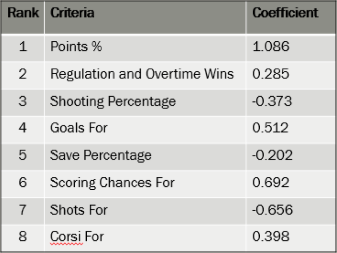
Starting off with all statistics I could collect for teams at Thanksgiving, I began to weed out less predictive variables until I landed on a group of 8. Using Recursive Feature Elimination (RFE), I was able to continually run the model and see which variables were deemed most predictive and should be included in the model. The factors as listed below were deemed most predictive, in order of importance 
to the model. 

While point percentage is the most predictive, other statistics like shooting percentage, save percentage, or goals for percentage provide a bigger picture perspective that allows for a better predictive capability for the machine learning model.

It has been determined that having higher shots for, shooting percentage, and save percentage all have a negative effect on whether or not you end up making the playoffs. For shooting percentage and save percentage, this is likely due to the fact that the model has identified a PDO like correlation in which teams with a lower save percentage and shooting percentage can be classified as “unlucky” and will eventually regress towards the norm. Additionally, the number of shots a team takes relative to the other team has a negative correlation with making the playoffs. This could be due to score effects that cause losing teams to typically generate more shots that are of lower quality. As the model shows, it is primarily high danger chances that are predictive of making the playoffs, not just any shot.

The Results

Running the model, 81.25% or 13 out of 16 playoff teams in a playoff spot as of March 1stwere correctly classified as playoff teams. Furthermore, an additional 2 teams (Columbus and Colorado) sat only 1 point back of a playoff spot. In contrast, picking the playoff teams at Thanksgiving would only result in a 68.75% success rate or 11 out of 16 teams. Furthermore, 3 teams that were in a playoff position at Thanksgiving are no longer in the playoff race in comparison to only 1 team (Buffalo) predicted by the model. 

Outliers

Particularly interesting decisions made by the machine learning model include the decision to not pick the Rangers to make the playoffs, despite leading the Metro at Thanksgiving, and the choice to select Vegas to make the playoffs despite a slow start.

One reason behind this choice could have been New York’s low number of ROW. With a mere 8 ROW in 22 games, the New York Rangers sat atop the Metropolitan Division mainly in part to their 4-0 record in shootouts. Seeing that the New York Rangers were playing so many close games, the model likely discounted the strength of the Rangers. Additionally, the New York Rangers had the 4thlowest corsi for %, 6thlowest shots for %, 9thlowest scoring chance for %. As for points for %, the Rangers were ranked at an underwhelming 13th in the league, but led the Metro since the Metro was a weak division and the Rangers had more games played. Given the Rangers low valuation across all these supporting criteria, the machine predicted that they would not make the playoffs despite their stronger points for % at Thanksgiving. 

As for the Golden Knights, despite holding the 29thbest point % in the league, Vegas was among the top 4 in the league in shots for %, corsi for % and scoring chances for %. Additionally, Vegas had the league’s lowest PDO (SH% + SV%) at 95.66. Given all these things considered, the model likely believed it was only a matter of time before the Vegas Golden Knights began winning.

Flaws in the Model

While my machine learning model appears to have the ability to out predict the strategy of picking all playoff teams at Thanksgiving, two main limitations of the model as highlighted above is the inability of the machine to pick teams based on the given playoff format, and the lack of data at various game states. 

Unaware of the NHL’s current playoff format, the model picked 9 Eastern Conference teams, and only 7 Western Conference teams. Without a grasp on the alignment of divisions within the league, the model is at a disadvantage when picking teams, particularly when specific divisions or conferences are more “stacked” than others. Therefore, there is the potential of the model picking an otherwise impossible selection of teams to make the playoffs.

Furthermore, data collected to be fed into the model was only even-strength data. While this provides a decent picture of a team’s capability, certain teams that rely on their power play, as the Penguins traditionally have, may be disadvantaged and discounted. Finding a way to incorporate this data into the model would likely provide a fuller picture and a more accurate prediction.

Final Thoughts

While the model I have created is by no means perfect, it provides a unique perspective into not only the importance of the first 20 or so games of the season, but also what statistics beyond wins are important in attempting to classify a playoff team. While the model appears to out predict the strategy of selecting all playoff teams at Thanksgiving, it will be interesting to see in years to come if there is a continued ability to classify playoff teams given Thanksgiving stats.

Statistics retrieved from Natural StatTrick

---

Keep up to date with the Queen's Sports Analytics Organization. Like us on Facebook. Follow us on Twitter. For any questions or if you want to get in contact with us, email qsao@clubs.queensu.ca, or send us a message on Facebook.

What makes a Top 10 pitcher?

By Josh Margles

In baseball statistics, an earned run average (ERA) is the mean of earned runs given up by a pitcher per nine innings pitched. I decided to take a deeper look to see what goes into the ERA of a pitcher. In this study, I divided all the qualified pitchers from the last five years into two groups; top 10 ERA and non-top 10, as a means to determine what makes a top 10 ERA pitcher.

Using four indicators; strikeout percentage, walk percentage, left on base percentage, and BABIP (batting average on balls in play) we can figure out the probability that a pitcher will finish in the top 10 in ERA. I ranked all the pitchers in the last five seasons by these categories, and put them into a big matrix of numbers based on their rankings. To indicate if they finished in the top 10 ERA category, I put a 1 for top 10, and a 0 for finished outside the top 10. I used each pitcher’s yearly rank instead of their actual numbers because each year’s top 10 is different. Therefore, it is important to compare numbers on a year- to-year basis.

Some of the chart looks like this:

To find a prediction, I used a program in R called XGBoost. XGBoost takes the information based on the previous data and tests to see if there is a pattern between where the pitcher finished in rank, and if he finished in the top 10 of ERA in the season. After running the numbers with different parameters on XGBoost we can determine two things. The program tells us which of the four stats is most indicative of a high ERA rank, and which pitchers were outliers (the model predicts the outcome).

First, let’s look at which stat is the most predictive in determining the rank. Surprisingly, LOB rank has the most impact on a pitchers ERA rank. Note that these aren’t percentages, rather they are used to show the relative importance in each stat in predicting ERA.

This chart shows that where the pitcher finishes in LOB percentage is the best predictor. Interestingly enough, the pitcher that had the highest LOB percent (he left the highest percentage of runners on base) each of the last five years finished in the top 10 in ERA. Also, out of the pitchers that finished in the top five LOB percentage, 20 out of the 27 (there was one three-way tie) finished in the top 10. The chart also shows that LOB rank and K rank are much more significant than BB rank or BABIP rank.

Next, let’s look at the predictive aspect of the model. I ran the model using a number of different combinations of test and training data, and then had it predict on the pitchers. The model predicted around 85 percent of the pitchers correctly. Now, let’s look at a few pitchers that the model incorrectly predicted and why this data was wrong.

Garrett Richards finished the 2014 season with a 2.61 ERA, which placed him 10th in the MLB. However, the model predicted that Richards would finish outside of the top 10 with those ranks. One explanation for why Richards finished with a good ERA is his HR rate. He had a 0.27 HR/9 rate in 2014, which was the lowest of any qualified pitcher in the last five years. So, while he allowed a lot of baserunners, not a lot came in because of the fact that he could keep the ball in the yard. Richards has been injured the last few years, but his success has been almost completely related to his home run rate.

Stroman in 2017 had an ERA of 3.09, which placed him 9th. What Stroman lacks in strikeouts, he made up for in his ground ball to fly ball rate, as well as his groundball percentage. This allowed Stroman to get easy outs without needing to strike everyone out. Since he got so many groundballs, most of the hits he gave up were singles, which limited the amount of earned runs. He also induced the most double plays in 2017, which helped him get out of innings without allowing any earned runs.

One problem with this model is that it treats everyone outside the top 10 as equals. In 2015, Scherzer had a 2.79 which was the 11th best in the MLB. Even though he finished with a great ERA, the reason he didn’t make it into the top 10 was because of the amount of HR he allowed. He gave up 31 HR which was the most in the NL. Even though he finished in the top 10 in these four stats, his home runs prevented him from being in the top 10 in ERA.

One of the more interesting results was that the model projects Fiers in the top 10 even though he had a 3.56 ERA, finishing 24th in 2018. The reason why his LOB rank is so good, while still consistently giving up runs, is because he gave up the second most HR/9 of anyone in the MLB. While the rest of his numbers look good, like Scherzer, home runs prevented Fiers from having an elite ERA.

Stats from FanGraphs, Baseball-Reference, and Baseball Savant

How important is winning a period in the NHL?

By Adam Sigesmund (@Ziggy_14)

Sometimes when I watch hockey on television, the broadcast will display a stat that makes me cringe. One of my (least) favourites is a stat like the one displayed just under the score in the screenshot below:

Most of us have noticed these stats on broadcasts before. I imagine they are common because they match the game state (i.e. the Leafs are leading after the first period), so broadcasters probably believe we find them insightful. However, we are all smart enough to understand that teams should theoretically have a better record in games that saw them outscore their opponents in the first period. In this case, whatever amount of insight the broadcasters believe they are providing us with is merely an illusion. Perhaps they also saw value in the fact that the Leafs were undefeated in those 13 games, but that is not what I want to focus on today. 

More generally, my primary objective for this post is to shed light on the context behind this type of stat, mostly because broadcasts rarely provide it for us. Ultimately, I will examine 11 seasons worth of data to understand how the outcome of a specific period effects the number of standings points a team should expect to earn in that game. Yes, this means there will be binning*. And yes, I acknowledge that binning is almost always an inappropriate approach in any meaningful statistical analysis. The catch here is that broadcasters continue to display these binned stats without any context, and I believe it is important to understand the context of a stat we see on television many times each season.

* Binning is essentially dividing a continuous variable into subgroups of arbitrary size called “bins.”In this case, we are dividing a 60-minute hockey game into three 20-minute periods. 

A particular team wins a period by scoring more goals than their opponent. I looked at which teams won, lost, or tied each period by running some Python code through a data set provided by moneypuck.com. The data includes 13057 regular season games between the 2007-2008 and 2017-2018 seasons, inclusive. (Full disclosure: I’m pretty sure four games are missing here. My attempts to figure out why were unsuccessful, but I went ahead with this article because the rest of my code is correct, and 4 games out of over 13K is virtually insignificant anyways).  The table below displays our sample sizes over those eleven seasons:

Remember that when the home team loses, the away team wins, so the table with our results will be twice as large at the table above. I split the data into home and away teams because of home-ice advantage; Home teams win more games than the visitors, which suggests that home teams win specific periods more often too. We can see this is true in the table shown above. In period 1, for example, the home team won 4585 times and lost only 3822 times. The remaining 4650 games saw first periods that ended in ties. 

We want to know the average number of standings points the home team earned in games after winning, tying, or losing period 1. This will give us three values: One average for each outcome of the first period. We also want to find the same information for the away team, giving us atotal of six different values for period 1. (This step is not redundant because of the “Pity Point”system, which awards one point to the losing team if they lost in overtime or the shootout. The implication is that some games result in two standings points but others end in three, so knowing which team won the game still does not tell us exactly how many points the losing team earned). Repeating this process for periods 2 and 3 brings our total to 18 different values. The results are shown below:

The first entry in the table (i.e. the top left cell) tells us that when home teams win period 1, they end up earning an average of 1.65 points in the standings. We saw earlier that the home team has won the first period 4585 times, and now we know that they typically earn 1.65 points in the standings from those specific games. But if we ignore the outcome of each period, and focus instead on the outcomes of all 13057 games in our sample, we find that the average team earns 1.21 points in the standings when playing at home. (This number is from the sentence below the table —the two values there suggest the average NHL team finishes an 82-game season with around 91.43 points, which makes sense). So, we know that home teams win an average of 1.21 points in general, but if they win the first period they typically earn 1.65 points. In other words, they jumped from an expected points percentage of 60.5% to 82.5%. That is a significant increase.

However, in those 4585 games, the away team lost the first period because they were outscored by the home team. It is safe to say that the away team experienced a similar change, but in the opposite direction. Indeed, their expected gain decreased from 1.02 points (a general away game) to 0.54 points (the condition of losing period 1 on the road). Every time your favourite team is playing a road game and loses period 1, they are on track to earn 0.48 less standings points than when the game started; That is equivalent to dropping from a points percentage of 51% to 27%. Losing period 1 on the road is quite damaging, indeed. 

Another point of interest in these results, albeit an unsurprising one, is the presence of home-ice advantage in all scenarios. Regardless of how a specific period unfolds, the home team is always better off than the away team would be in the same situation.

I also illustrated these results in Tableau for those of you who are visual learners. The data is exactly the same as in the results table, but now it’s illustrated relative to the appropriate benchmark (1.21 points for home teams and 1.02 points for away teams).  

Now, let’s reconsider the original stat for a moment. We know that when the Leafs won the first period, they won all 13 of those games. Clearly, they earned 26 points in the standings from those games alone. How many points would the average team have earned under the same conditions? While the broadcast did not specify which games were home or away, let’s assume just for fun that 7 of them were at home, and 6 were on the road. So, if the average team won 7 home games and 6 away games, and also happened to win the first period every time, they would have: 7(1.65) + 6(1.53) = 20.73 standings points. Considering that the Leafs earned 26, we can see they are about 5 points ahead of the average team in this regard. Alternatively, we can be nice and allow our theoretical “average team”to have home-ice advantage in all 13 games. This would bump them up to 13(1.65) = 21.45 points, which is still a fair amount below the Leafs’ 26 points. 

One issue with this approach is that weighted averages like the ones I found do not effectively illustrate the distributionof possible outcomes. All of us know it is impossible to earn precisely 1.65 points in the standings —the outcome is either 0, 1, or 2. An alternative approach involves measuring the likelihood of a team coming away with 2 points, 13 times in a row, given that all 13 games were played at home and that they won the first period every time. We know the average is 13(1.65) = 21.45 standings points, but how likely is that? It took a little extra work, but I calculated that the average team would have only a 3.86% chance to earn all 26 points available in those games. (I did this by finding the conditional probability of winning a specific game after winning the first period at home, and then multiplying that number by itself 13 times). Although the probability for the Leafs is a touch lower than this, since there is a good chance a bunch of those 13 games were not played at home, you should not allow such a low probability to shock you; 13 games is a small sample, especially for measuring goals. There is definitely lots of luck mixed in there. 

This brings us back to my original anecdote about cringing whenever I encounter this type of stat. Even if we acknowledge its fundamental flaw —scoring goals leads to wins, no matter when those goals occur in a game —the stat is virtually meaningless in a small sample. Goals are simply too rare to provide us with much insight in a sample of 13 games. Nevertheless, broadcasters will continue displaying these numbers without context. This article will not change that. So, the next time it happens, you can now compare that team to league average over the past eleven seasons. Even if the stat is not shown on television, all you need to know is the outcome of a specific period to find out how the average team has historically performed under the same condition. At the very least, we have a piece of context that we did not have before.